How does raster data work in a lakehouse?

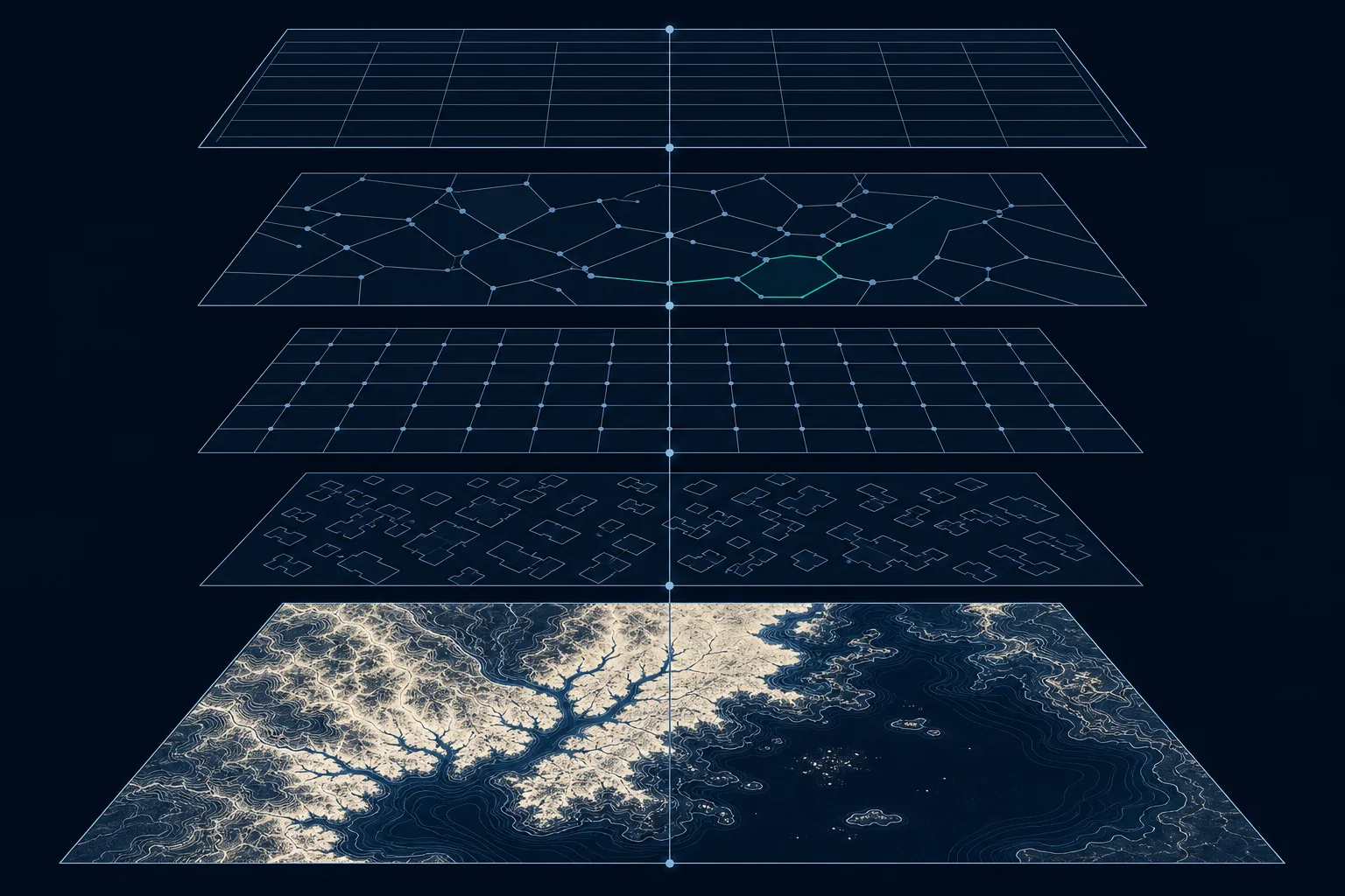
Raster data is the least table-shaped data an organization owns. An image is a grid of millions of pixels, and a climate dataset is a stack of such grids across decades. Nothing about that shape fits naturally into rows and columns, and yet the decisions this data supports, property risk, crop condition, storm exposure, run through the same governed platforms as everything else the business trusts.

Teams usually resolve the mismatch in one of two bad directions. Some serialize pixels into tables and pay for storage and query patterns the data was never meant for. Others leave imagery in specialist silos, ungoverned and invisible to the platform, connected to it by exports nobody audits.

Production systems converge on a third arrangement: the pixels stay in files, and tables carry everything the platform needs to know about them. This guide walks through how that works, from acquisition to serving.

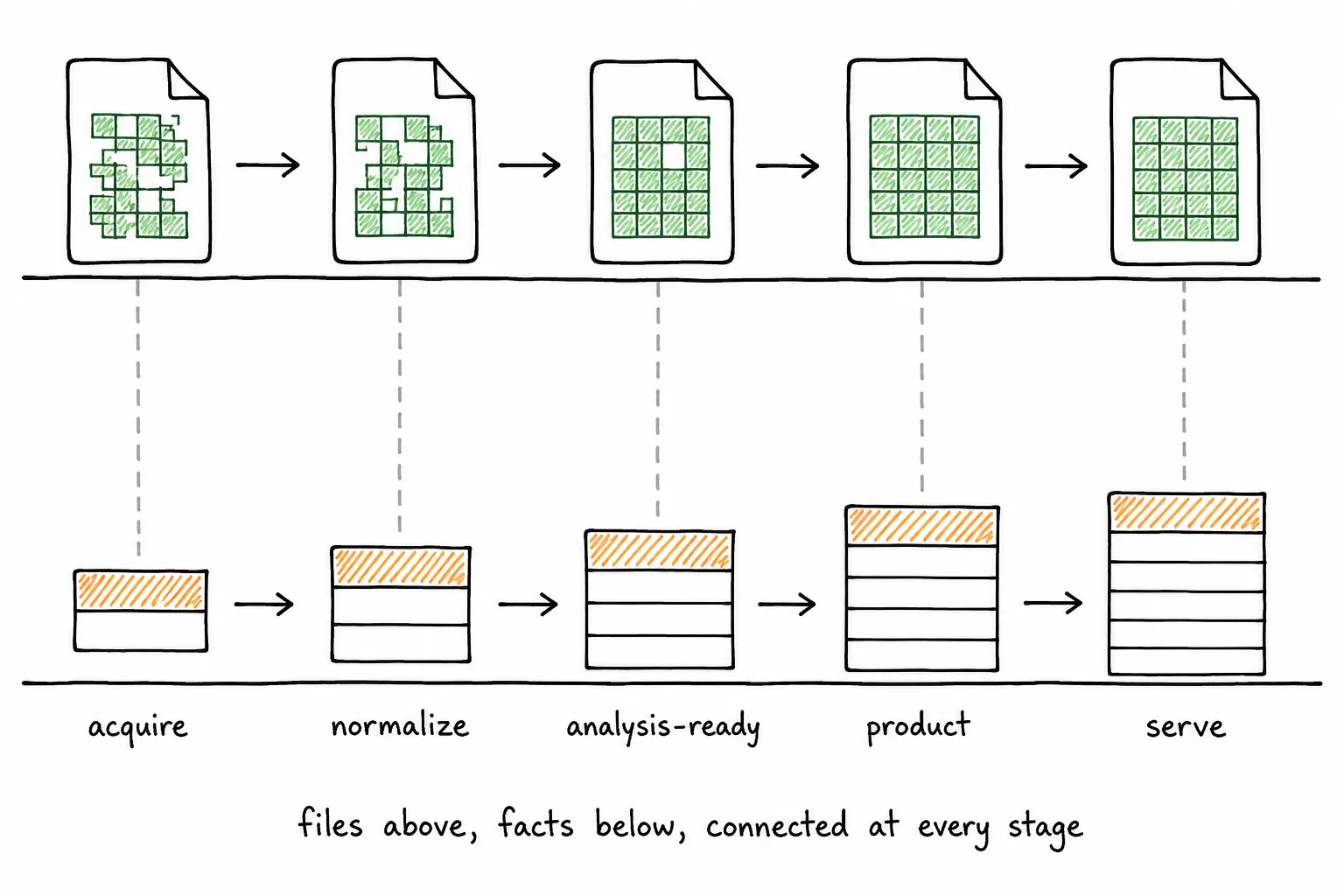
The whole pipeline in one drawing. Pixels move through files on the upper rail, the facts about them accumulate in tables on the lower rail, and the two rails stay connected at every stage.

What does it mean to make raster data queryable?

Queries never touch pixels. A platform filters and joins rows, so raster participation depends on a catalog table that describes each image or grid: where its pixels are, what place and time they cover, how they are encoded, and whether they passed validation. The pixels themselves may remain in object storage.

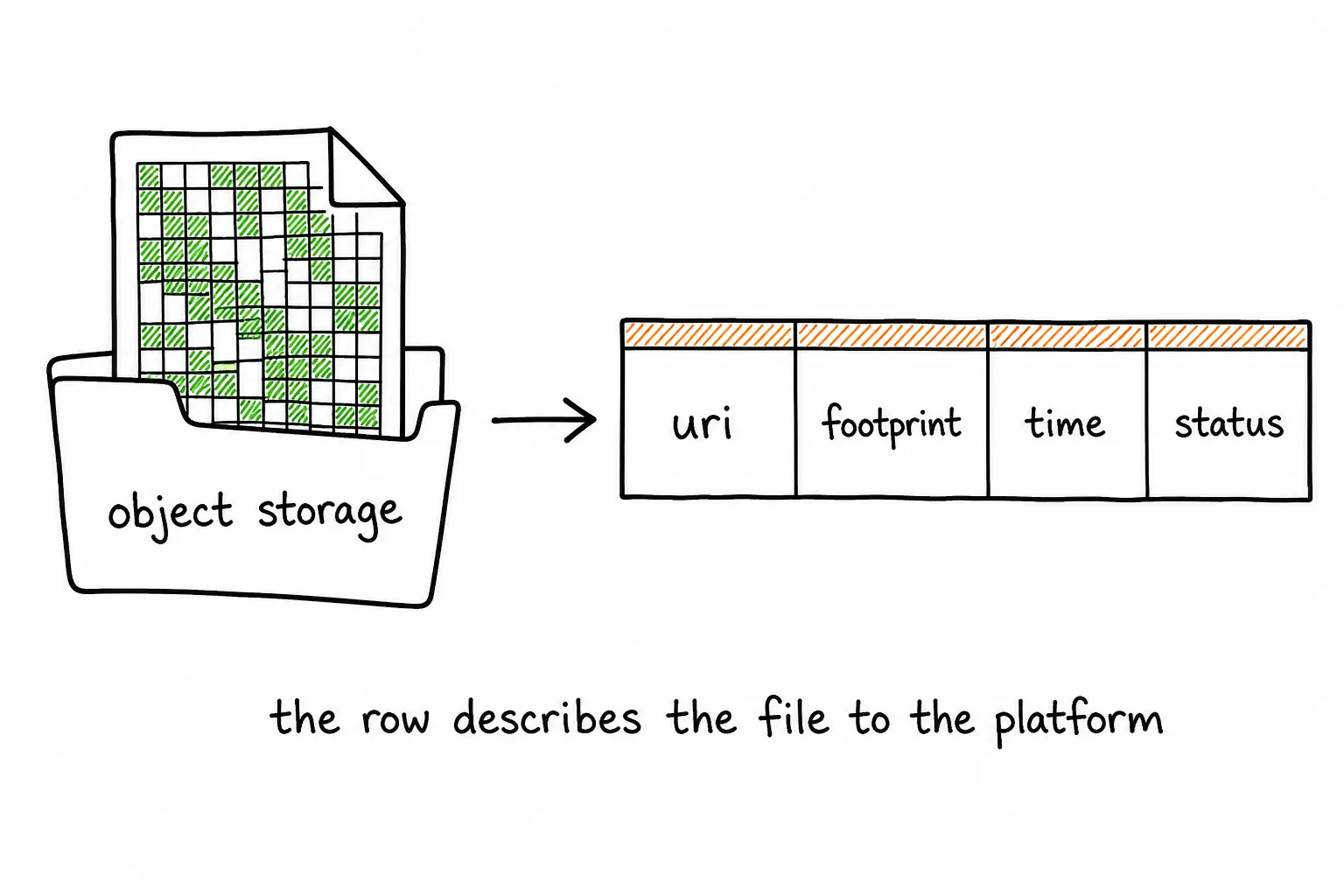
The pixels stay in the file. The catalog row describes the file to the platform, and the row is what queries touch.

This design separates two concerns. Object storage holds large binary arrays efficiently. Managed tables expose the metadata and derived measurements that analysts, applications, and pipeline jobs need. A query can find all cloud-free scenes intersecting a property portfolio during a date range before any job opens the corresponding image files.

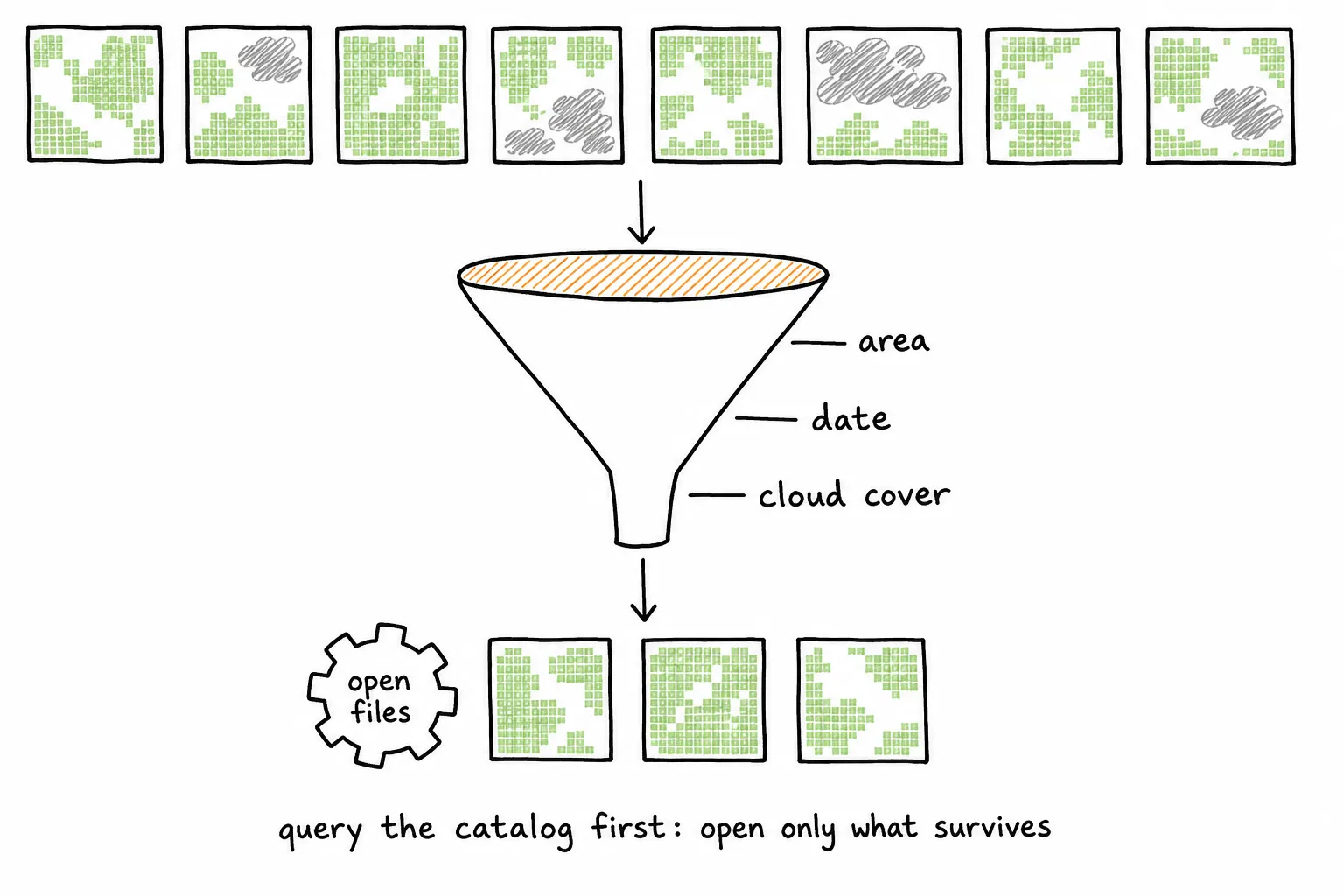
Query the catalog first. Only the scenes that survive the filters are worth the cost of opening.

How does raw imagery enter the lakehouse?

Everything downstream inherits what acquisition preserves or loses, which is why the process stays controlled. The pipeline records the source, original object identifier, acquisition time, receipt time, checksum, license terms, and storage location, and it keeps the original file unchanged whenever the license and retention policy permit.

Checksums reveal incomplete transfers and duplicate deliveries. Stable source identifiers support repeatable updates. A manifest records which objects arrived in each acquisition run. These controls make it possible to answer a basic operational question: exactly which provider data was available when a downstream product was built?

A source file can be invalid, unexpectedly large, or encoded differently from the provider specification. Acquisition therefore includes validation and quarantine. Failed objects stay visible in run reporting but do not proceed into trusted data states.

Which raster metadata belongs in tables?

The schema follows from what the platform must do with the rows: discover scenes, validate them, partition work, and trace lineage. Common fields include the storage URI, spatial footprint, bounding box, coordinate reference system, pixel dimensions, band definitions, no-data values, acquisition time, processing level, source identifier, checksum, and quality status.

Teams should also record fields specific to the decision the imagery supports. Optical imagery may need cloud cover and sun angle. Elevation data may need vertical datum and resolution. Weather grids may need forecast issue time, valid time, variable, and units.

The table schema should distinguish provider metadata from values calculated by the pipeline. That distinction helps reviewers trace discrepancies and decide which fields require recalculation after processing logic changes.

How does imagery become analysis-ready?

Two scenes from the same provider can differ in projection, resolution, and cloud handling, and a workload needs them comparable. Versioned transformations get them there, which is what analysis-ready means in practice. Typical steps include reprojection, band selection, no-data normalization, resampling, clipping, tiling, and quality masking, in a sequence that depends on the source and intended analysis. These transformation stages follow the geospatial lakehouse medallion architecture.

A shared grid or tile scheme can make distributed work predictable. Each output partition receives a stable spatial key. Jobs can process independent partitions, retry failures, and join raster-derived measurements to vector features through a documented crosswalk. The chosen grid resolution must preserve the detail required by the business decision. A convenient global index can still be too coarse for parcel-level risk.

Analysis-ready data should identify the transformation version and every source object used. Reprocessing creates a new version or release rather than silently changing a prior result.

How do pixels become governed table values?

The business does not ask about pixels. It asks about fields, buildings, grid cells, and scenes, so the pipeline computes measurements at those grains, and the measurements, not the pixels, are what enter governed tables. Examples include vegetation condition by field, flood depth by building, temperature by grid cell, or image quality by scene. Each row combines a business or spatial identifier with the measurement, units, observation period, source reference, and processing version.

The output needs a clear contract. A flood depth column should state whether it represents maximum depth, mean depth, or a percentile. A building exposure record should state how pixels were selected when a footprint crosses several cells. These definitions turn a technical result into a reusable data product.

Quality checks can reject impossible ranges, missing units, incomplete coverage, duplicate keys, or unexpected changes from the previous release. Accepted rows enter a governed product table with a named owner and refresh policy.

When should pixels remain in files?

Serializing every pixel into rows is possible and usually pointless. Large imagery archives, multidimensional climate arrays, and intermediate tiles are read as arrays, windowed and resampled, access patterns that rows serve badly, so those pixels stay in files. A geospatial lakehouse does not require serializing every pixel into a table.

The files still participate in governance. Catalog rows provide discovery and access paths. Storage permissions protect the underlying objects. Lineage connects source files to transformations and derived tables. Retention policies state which intermediate files can be rebuilt and which source files must be preserved.

How are raster outputs served to users and applications?

A zonal statistics table, a map tile, a feature store row, and a partner share can all express the same accepted product. Each consumer gets the representation that fits how it works: analysts use SQL tables of zonal statistics, models read partitioned feature tables, maps use image tiles, applications call a low-latency service keyed by asset or location, and partners receive a governed table share.

Their physical formats differ, while their business meaning and release identifier remain aligned. Treating serving as a deliberate pipeline stage prevents an application cache or map tile store from becoming an undocumented source of truth.

About the author

Sean Knight is a serial entrepreneur in the San Francisco Bay Area who builds products and companies around AI and geospatial data. He opened his first business, a retail computer shop, at 17, then began his career as an astrophysicist. From there he moved into remote sensing and machine learning, eventually flying drones over glaciers in Alaska and New Zealand to build 3D point clouds. Today he runs LakeGeo, consults on AI, and builds AI agents that run geospatial pipelines on platforms like Databricks. Find him on LinkedIn.