How do you build a geospatial lakehouse on Snowflake?

Many teams already keep business data, reference data, and analytical products in one governed warehouse. Adding location data raises a practical concern: some spatial workloads fit the warehouse well, while others bring specialized files, libraries, and processing requirements.

A geospatial lakehouse must preserve common governance without forcing every workload through the same execution path. The central design decision is where each type of spatial work should run and who will operate the connections between systems.

The Snowflake approach starts with a governed center for vector analysis. It then adds operated attachments for workloads that native warehouse services do not cover.

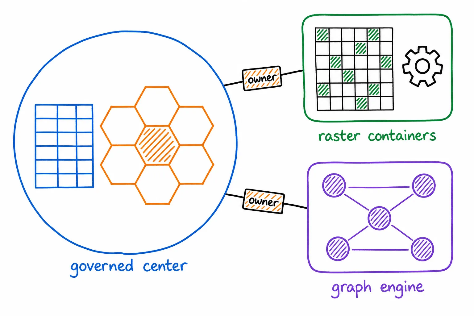
The governed center holds the vector path. Raster and graph work run as operated attachments, each boundary with an owner.

Which spatial work belongs inside the warehouse?

Most location analysis begins with points, lines, polygons, and relationships such as intersection or distance. Snowflake stores these features in native GEOGRAPHY and GEOMETRY columns. GEOGRAPHY uses a spherical coordinate model, while GEOMETRY uses a planar coordinate model. Spatial SQL supplies constructors, predicates, measurements, transformations, and aggregates for working with both types.

H3 is a hexagonal discrete global grid system. Native H3 functions assign features to cells, calculate coverage and neighbors, move through the grid hierarchy, and reduce the candidates examined by spatial joins. These capabilities keep the common vector path inside governed tables and SQL.

Other spatial data needs an attachment. Raster data organizes measurements in a grid of cells. Snowpark Python runs Python code close to warehouse data, while Snowpark Container Services runs custom software and graphics processing unit (GPU) workloads in managed containers. Teams can use these services for raster processing, specialized libraries, and other work that does not fit native SQL.

Iceberg support connects the warehouse to data stored in an open table format. That compatibility does not make the architecture independent of Snowflake. Governance and much of the execution still depend on Snowflake services, so the Iceberg boundary should be an explicit architectural choice.

How do the six lakehouse layers map to Snowflake?

The Geospatial Lakehouse Stack separates the platform into six layers that can be assigned clear services and owners.

Ingestion brings data into the platform. Snowpipe loads arriving files, Snowpipe Streaming accepts live records, and COPY INTO handles batch loads. Openflow supplies managed connectors and change data capture, the process of recording inserts, updates, and deletes from a source system.

Storage and governance hold spatial assets and control their use. Native tables or Iceberg tables store tabular spatial data. Stages hold raster and scientific files. Horizon Catalog applies governance, while Secure Data Sharing and Marketplace distribute data without creating unmanaged copies.

Spatial compute handles the analytical work. Native spatial SQL and H3 cover vector operations. Snowpark Python or Container Services process raster data. Graph analysis runs through Snowpark or an external engine.

Machine learning and AI manage features, models, and specialized inference. Snowflake ML Feature Store records reusable model inputs, and Model Registry manages trained models. Container Services supports custom training and inference. Cortex AI functions and Cortex Search provide additional AI services.

Orchestration keeps data products current. Dynamic Tables maintain query results as their source data changes. Tasks and Streams coordinate imperative pipelines, while Snowpipe Streaming continues to ingest live records.

Consumption places governed results in front of people and applications. Snowsight supports warehouse analysis, and Streamlit in Snowflake hosts data applications. Cortex Analyst and Snowflake Intelligence provide analysis interfaces. Hybrid Tables support operational lookups, and Secure Data Sharing distributes products to other accounts.

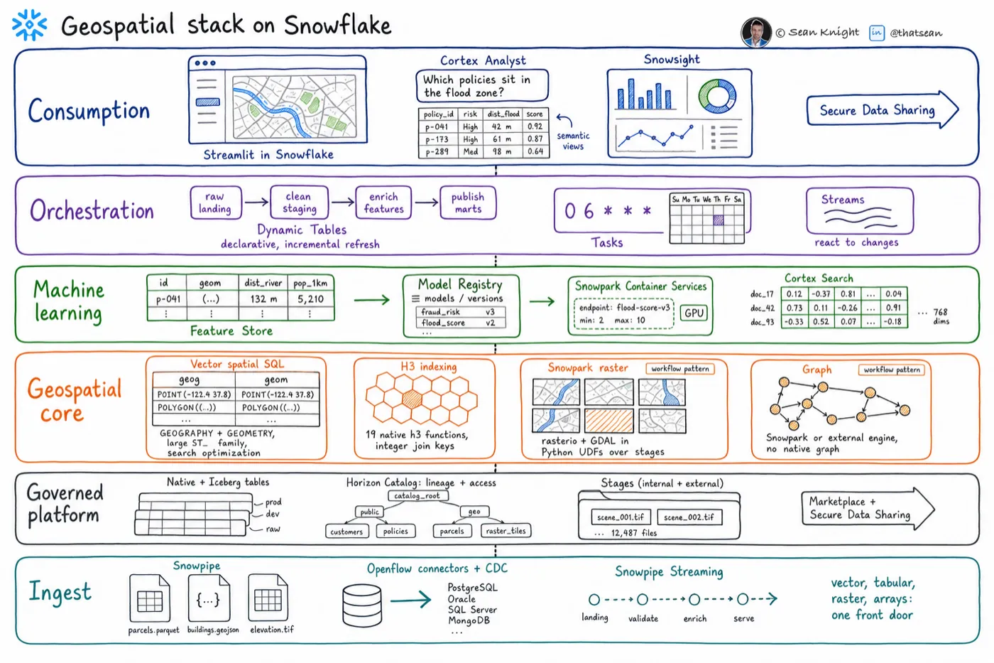
The six layers of the Geospatial Lakehouse Stack on Snowflake, service by service.

How does data move from acquisition to a governed product?

The Geospatial Medallion Architecture turns the platform layers into a sequence of managed data stages.

In the acquire stage, Snowpipe and COPY INTO collect files. Openflow connects managed sources, while external access reaches provider interfaces. Marketplace listings can replace file acquisition when a needed reference dataset is already available there.

The bronze stage preserves the source. Files remain in write-once stage paths, and bronze tables retain original tabular values. This stage creates a stable record that later processing can revisit.

The silver stage prepares data for analysis. Snowpark or Container Services creates raster files optimized for cloud access. Spatial pipelines validate vector geometry and add H3 indexes where appropriate. Dynamic Tables can maintain these analysis-ready tables as source data changes.

The gold stage publishes data with defined meaning and ownership. Gold tables become governed products rather than intermediate pipeline outputs. Reusable machine learning features and models are registered with Snowflake ML services.

The serve stage connects those products to users and other systems. Snowsight and Streamlit support analysis and applications. Hybrid Tables handle operational lookups. Secure Data Sharing and Marketplace distribute approved products.

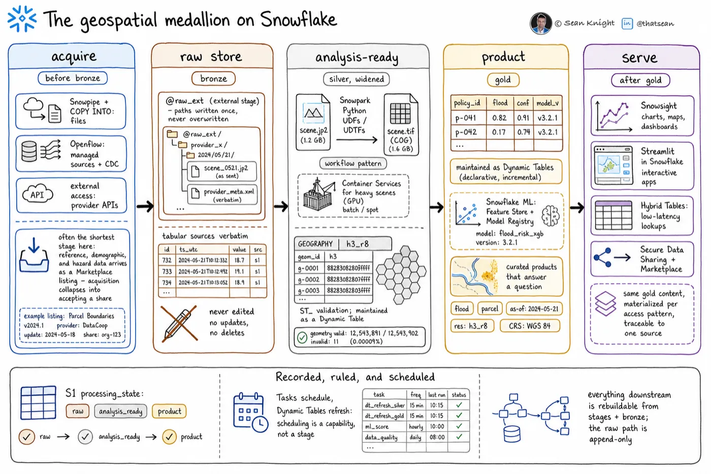
Snowflake services assigned to each stage of the geospatial medallion.

Where does this architecture have the clearest advantages?

The native vector foundation reduces the number of systems involved in common spatial analysis. Geometry storage, spatial predicates, measurements, aggregation, and H3 filtering can remain within warehouse governance.

Marketplace can supply reference data without a separate file acquisition process. Secure Data Sharing provides a controlled path for distributing finished products. Together, these services connect acquisition and publication to the same governance model.

Dynamic Tables offer a concise model for incremental silver and gold pipelines. Teams describe the desired result while the service maintains it as inputs change. When native SQL is insufficient, Container Services provides a managed execution path for custom raster libraries and GPU work.

Which limits require explicit operating decisions?

Snowflake has no native raster or point-cloud engine. A point cloud is a collection of spatial measurements that commonly represents three-dimensional surfaces. Raster and point-cloud processing therefore introduces code and operating boundaries outside native spatial SQL.

The platform also lacks native topology for maintaining spatial relationships, graph analysis for connected networks, routing for selecting paths, and linear referencing for locating events by distance along a line. These workloads need Snowpark, containers, or an external engine with a named owner.

Hard sub-second geofencing usually needs a stream processor ahead of Snowflake. Geofencing means determining whether a moving object has entered or left a defined area. Snowflake search optimization, container workloads, and repeated scans of large spatial datasets also require cost testing against the actual workload.

Where should a team begin?

Every workload outside the governed center adds an operating boundary that someone must own. Begin with the vector path in native spatial SQL and H3. Introduce raster, point clouds, topology, graph processing, routing, or specialized libraries only once each attachment has an operator, a governed data boundary, and a clear reason to exist.

The formal Snowflake page of the LakeGeo architecture provides the service-by-service reference. Companion articles cover the same build on Databricks and Google Cloud.

Keep common vector analysis in the governed center, and name the owner of every workload that must run outside it.

About the author

Sean Knight is a serial entrepreneur in the San Francisco Bay Area who builds products and companies around AI and geospatial data. He opened his first business, a retail computer shop, at 17, then began his career as an astrophysicist. From there he moved into remote sensing and machine learning, eventually flying drones over glaciers in Alaska and New Zealand to build 3D point clouds. Today he runs LakeGeo, consults on AI, and builds AI agents that run geospatial pipelines on platforms like Databricks. Find him on LinkedIn.